A few years ago, I tried my hand at the, now retired, CAPTCHA Forest CTF, which was part of the nullcon HackIM 2019. I wanted to solve it using computer vision and machine learning. This started me on a path of discovery and incremental improvements that finally resulted in capchan, a generic CAPTCHA to text tool.

This post is broken into four parts:

• The first CTF
• The second CTF
• Neural Network Fundamentals
• Creating capchan

ATTEMPT_ZERO

Starting the CTF – I connected to the netcat instance, but after staring at hexadecimal, I immediately closed it and moved on to try another CTF.

That was my first experience with Image Classification, and sure, some might call it an “unsuccessful attempt”. However, I remained optimistic. A while later I set my sights on it again, failed to install some dependencies in Python – moved on to another CTF. At this point, we could definitely call it an unsuccessful attempt.

Other than noting that I should use venv a bit more, I didn’t fully commit to solving this CTF. That’s more so that I wanted to get the easy points out of the way for my leaderboard chasing, rather than spending a lot of time on a few points. That said, the concept remained super interesting and I was itching to return to it whenever time allowed.

Sensecon time, Matthew and his doppelgängers, Ethan & Adriaan, suggested “Image Geolocating through AI” as our 24 hour hackathon idea. Not just did I join the team to be with Me, Myself and I (Ethan and Matthew) I knew it would benefit me in the long run for solving the CAPTCHA CTF. One Sensecon and a few dedicated research weeks later – this is where I am.

CAPTCHA_ONE (foreshadowing with one here)

Unfortunately, my fellow buzzword enjoyers – for the first CTF AI/Machine Learning wasn’t needed to retrieve the flag. However, I’ll give you the lay of the land here.

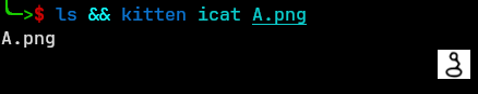
So what does the CTF look like?

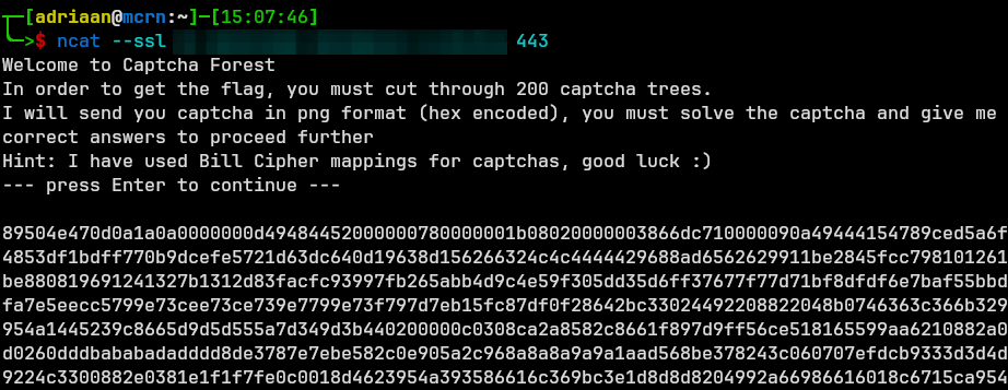
Not exactly the most attractive ‘image’ related CTF.

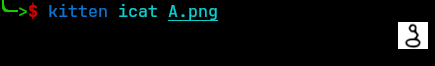
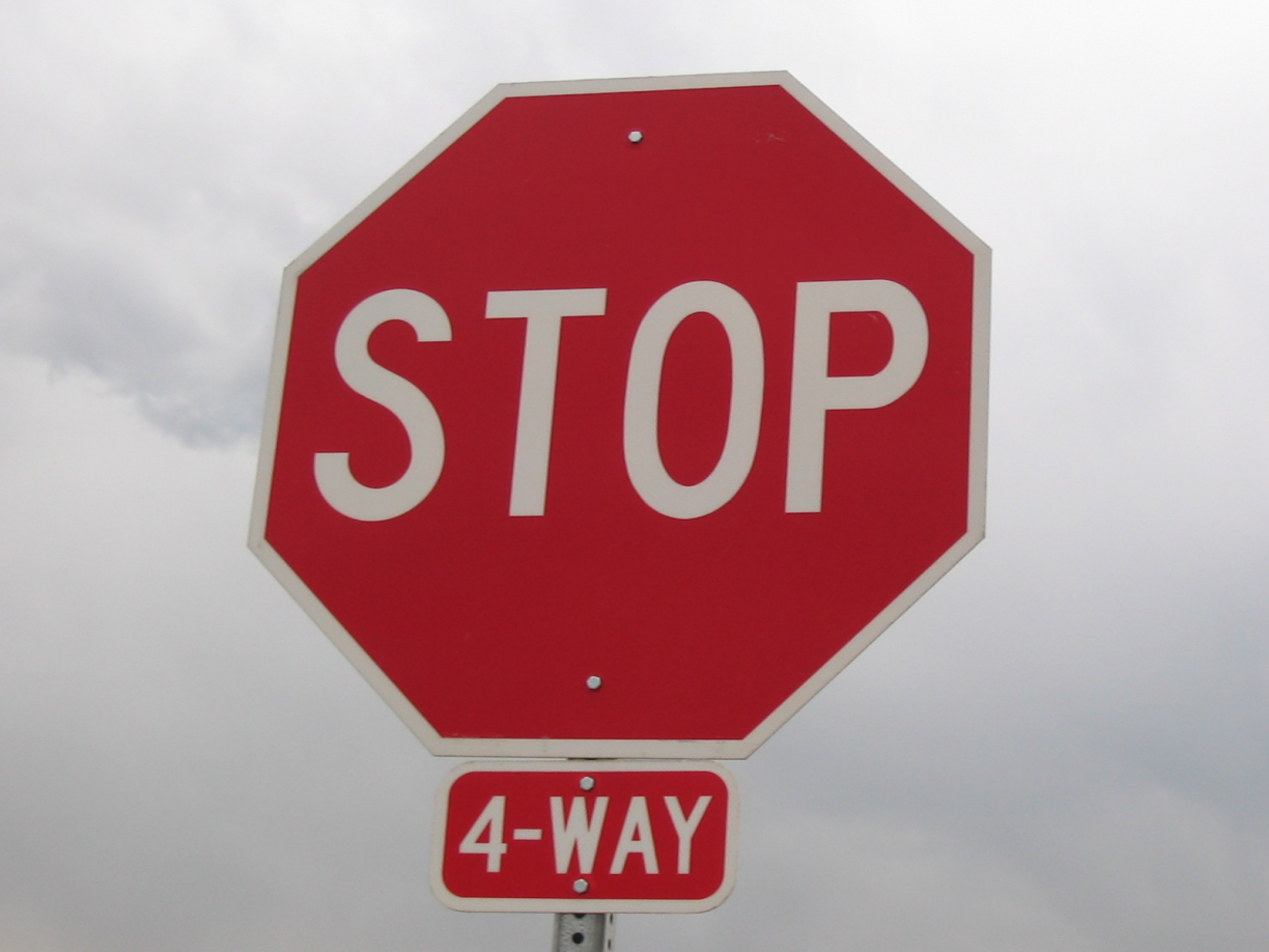
What’s happening? We connect to the instance using netcat, thereafter; the prompt states to solve the CAPTCHA 200 consecutive time in order for the flag to be given. The image is given in hexadecimal format. Viewing the image:

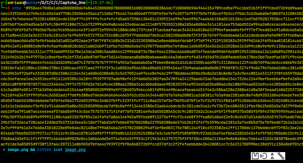
From this, we can see that my terminal is cool and can display images, but also that the CAPTCHA is some sick joke of a hieroglyphic. Luckily the prompt was generous enough to provide the mappings as Bill Cipher, from Gravity Falls, substitution cipher.

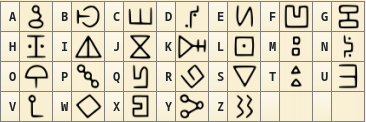
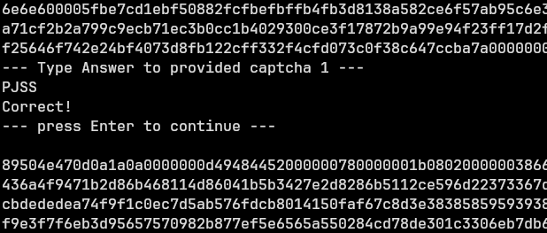
Referencing the previous image, the CAPTCHA code is FBTP, easy peasy – lemons got squeezed. The issue is I had to solve this 200 times. The clear answer was automation – although, I truly believe that the devs that made CAPTCHA Forest underestimate my tenacity to manually do this 199 more times – I decided to ‘play the game’.

Rinse and Repeat

How could I automate this? Checksum! Make a checksum of the image, since it will always be the same image for the same alphabetic characters. With this, one could connect to netcat, retrieve the image, make a checksum of the image and compare to the existing values to find the four character value, submit it back over the exiting netcat session – rinse and repeat. That’s probably what the ‘smart people’ would have done, but not around these parts. I wanted to solve this being as ‘close’ to the image as possible. So what did I decide on?

I decided to complete the challenge by using the pixel values, which is easy enough considering that the colour of the image would not determine the value of the characters. Solely taking pixel position into account, what I did was, once again, use the remote server to retrieve all the images until I had the full alphabet of ciphers. Then convert the images to black and white – just in case there were some dark spots or other values that could mess up the pixel data.

The other half of this was to make a script to retrieve the images from the server over netcat and compare pixel data, matching images would then be given the correct value and resubmitted over netcat until 200 iterations has been made.

TL;DR:

1. Take the hex over netcat and change it to a png.
2. This large image will have four symbols, so split it into four images instead, making it one symbol per image.
3. Determine the matches for each image and compile a four character code.
4. Send this back to netcat, and redo steps one through four.

More Visual

I now have Bill Cipher symbols as the images. A set of four symbols in a single image, which has now been made four images with a single symbol each. Why do it this way? We’ll, I am, in a way, hardcoding a checksum in a different way – with pixels. But having to test four images against 26 characters each is a lot better than checking against 26^4 or 456,976 possible combinations. Remember that I first have to define the value of each image since that the point of all this, and I am more than willing to do it 26 times, rather than 456,976 times over.

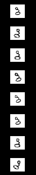
25 more times of the above and offline data collection complete. What remains is splitting the image from netcat into four parts to the same size as the offline images and compare. Since the CAPTCHA consistently provides the symbols (no rotations, distortion, etc) I should be able to get a 1:1 match.

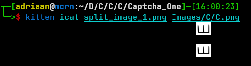
Below I have an example of my offline image I retrieved from netcat and an image from a more recent netcat interaction.

To visualise the above a bit more, this is what the script “sees” when comparing both images.

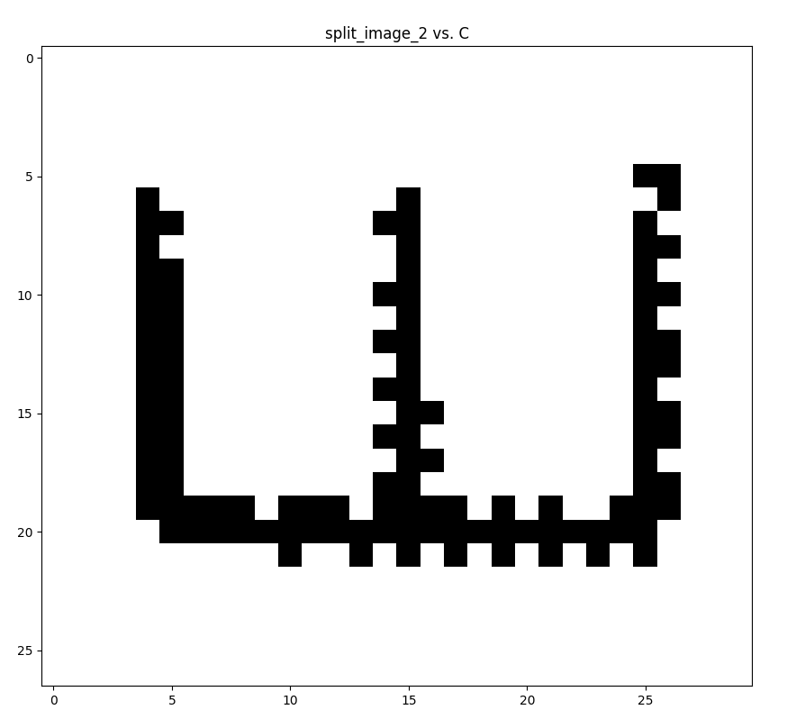
So with the 1:1 match, what’s left to do is have the script send the values of each split image to netcat and repeat the process 200 times, while, of course, combining the image results in a single four character code.

I made the scripts one by one for each problem and then added them all together to get to this point. And by adding them all together I mean this:

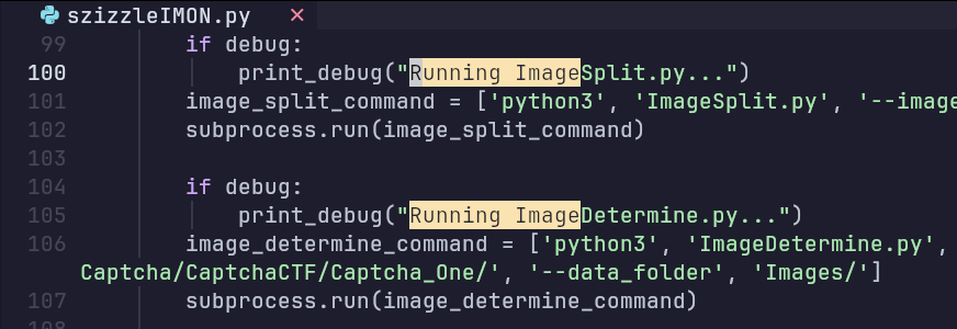
I am so sorry for those who code in Rust and Haskell – that they had to witness the abomination of what I have spawned in Python. Sidenote: When one gets bored they tends to add script flags and coloured output… Also, yes. My script is called szizzleIMON – Szymon told me to use tesseract in standup and this was my retaliation to his good idea.

Most of these scripts are simple and specific to the CTF, like connecting to netcat, taking the image, splitting it and sending it back to netcat (In a single script of course, lol). The most important thing is how the images were processed and compared:

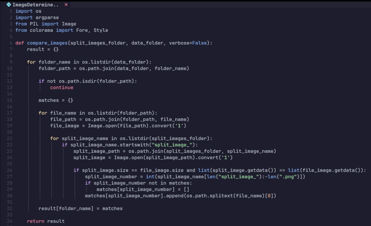
The compare_images function loops through each folder in my dataset. It takes these images and converts it to black and white, in case there isn’t any noise. It uses PIL to open each image then compares the size and pixel data to find a 1:1 match.

The link to the full code for both CAPTCHA CTFs is in the GitHub repo. Both CAPTCHA CTFs?

CAPTCHA_TWO (dun dun duuun)

To my absolute shock, when I submitted the flag, another CTF popped up – with some aura might I add, with its name being “Captcha Forest Harder”.

So why is it “Harder”? I had a quick glance at the new netcat instance and the description read; This challenge needs to be solved 120 times out of 200 tries to output the flag. I’ve never read anything scarier (other than the word “boo”).

Otherwise, the description and task was mostly the same. Have a look at the first CAPTCHA’s letter A:

Versus the new CAPTCHA’s letter A:

The images are distorted at random with noise added and rotation added to the mix. Making a checksum of something random is a bad idea and you would most likely not find two exact same images within your lifetime.

This completely voids my previous script. Now comes the Sensecon part, remember the thing with “Image Geolocating through AI” I did with my twins, Ethan and Matthew. Like a time traveller going back in time to ensure the creation of Linux – I predicted that I would use the newfound knowledge from Sensecon.

I decided to go with Image Classification for this CTF. This would use AI and Machine learning to guess the closest image in the dataset to the given image. This is thanks to TensorFlow in Python. In Sensecon our team described this as “dark magic”. Essentially you pre-process the image, provide a dataset to train a model and use the model according to the dataset. One thing from this; where do we start with AI stuff. This is why we called it dark magic – we don’t do the AI stuff. At least not the Math of it, but I’ll have you stare at some regardless.

Computer Vision

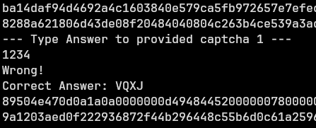
An important concept to understand is “computer vision” – we might see text and shapes in pictures, but computers just see this binary and at most highlight hex colour codes and pixel positions. It’s easy to get frustrated that a computer won’t be able to tell you that this is a stop sign.

You might think it’s a red octagon with the word “stop” in it, therefore; it should be simple enough for a computer to identify. However, let’s review how a computer see’s this.

It doesn’t ‘see’ like humans do. Even if it could ‘read’ the text on the stop sign in the image – it has to be perfect. The above image does not have the words perfectly flat to the viewer, therefore the letter “S” would have pixels missing at the top and additional pixels at the bottom, due to the angle its being viewed from. The perspective completely changes the letter and it’s no longer a perfect “S” to a computer. If its not a 1 its a 0, and small changes to us would be monumental for a computer.

Think of computer vision as trying to prove a line is a straight line. It’s easy to see a straight line, but how do you prove it? You can’t put a ruler on the screen and have the computer affirm that the line is in fact straight. Instead, there is a set way to prove this, i.e.: y=mx+c. Following this way of thinking is the key to solving the issue we have.

Dark Magic

I wasn’t happy with merely calling it “dark magic”, so I looked into how it works and detailed it below. But, you don’t need to know how it works to do the CTF, except for fine tuning a few things. The Nerdy stuff starts below under “Neural Networks”, which is a loaded statement, implying that this, currently, is not Nerdy.

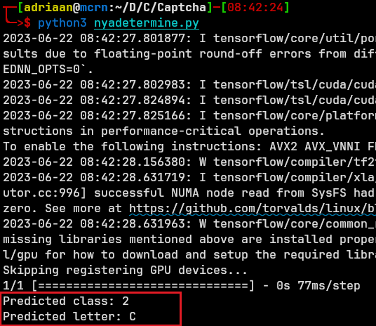
Enough yapping and let me show you what I did. I could recycle the script to connect to netcat, get the hex and change to images of four. Then finally sent it back. Now all we need to focus on is determining the symbol values.

First things first, let’s update the script name from szizzleIMON.py to szizzleIMONGHARD.py (This guarantees luck and it’s important you know what I call my scripts. The G in front of GHARD is supposed to mimic the accent of John, the greek). What I need is the following:

1. Dataset.
2. Creating and training a model.
3. Using the model. 

The Numbers

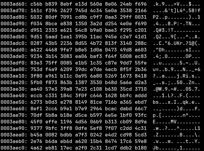
I need two types of data for my dataset; training data and validation data. Luckily they made it easier for me on this CTF.

After an incorrect value was given, the instance would provide the correct value. So I made a script to capture the hex, send “1234” as the answer, capture the corrected answer and named the hex file to the corrected value.

After using the CTF as a source of collecting datasets, In total I had roughly 7000 training data images and 4000 validation data images. Its important that the data had to be different images as the model needs it to verify its accuracy by testing against images it has not ‘seen’/processed before.

To create/train a model I used TensorFlow’s dark magic.

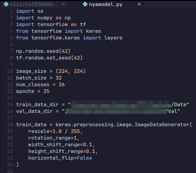
You might be thinking “Small script for AI and machine learning”. Well yes, that happens in the background and we just pre-process the image. TensorFlow is the reason why this blog is not about calculus and extreme values. We set the batch size, which is the number of samples that propagate through the neural network before updating the model. Specify the number of classes. Epochs, which you can think of is the amount of times the entire process will iterate (More epochs does not always mean better, there is a limit with the amount of data we provide.). Provide the training data and the validation data. I kept the image pre-processing low, since most of my data is already in unforeseen (rotated, distorted) format. The rest of the code was just moving the data, specifying training parameters and saving the model.

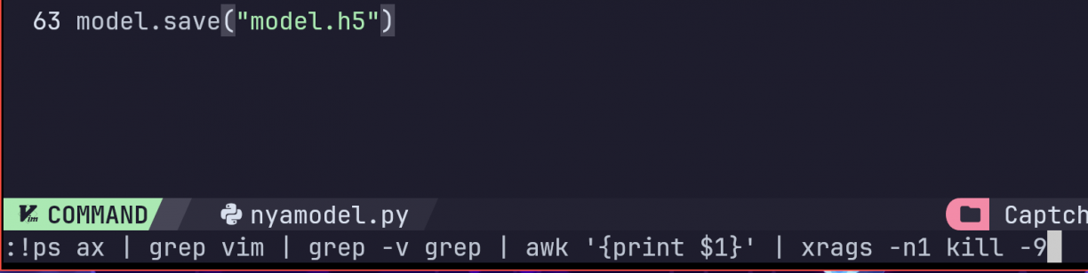
This will spit out the model for us to use in a .h5 format. Sidenote: did you know you can generate this model.h5 to have a shell inside of it? There were some office shenanigans where we added a shell inside the model and everyone who ran it got shelled. The model.h5 itself is not human readable so not something you see at first glance.

What remains was to specifying images to test against, ensuring the classes are defined exactly as they are in the model then saving this output.

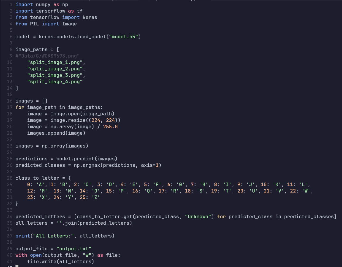
You might be wondering why I am saving this to output.txt. Keep wondering.

Sidenote: The contents of output.txt had control characters in them. I found this out on the first CTF and couldn’t figure out what was wrong. When I cat the file, the letters seemed correct and it was only until I opened it in vim, when I saw these characters (I had to restart my pc after this, because I couldn’t exit vim).

Some Results

Testing this scripts accuracy with a model that had 50 Epochs and a Noticeable Pre-Processing of images (Such as flipping the image).

This might seem good, but at most this guessed 25 images correct from the CTF before getting 80 more wrong and failing the attempt.

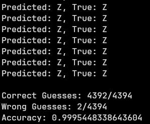
I tested the accuracy beforehand as you can see with the above image, which seemed deceivingly good. The problem was that the images I tested the accuracy with were recycled from images I had trained against. The dark magic section and later parts explain in more detail why this deception happens.

After ensuring the dataset had unique values exclusively, I created a model once more. At the end I found 25 Epochs and minimal to no image pre-processing to provide the best accuracy.

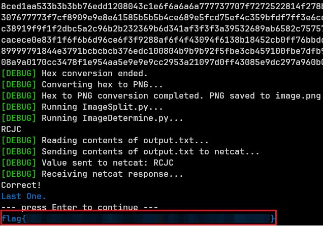
With this new accuracy this is what I got from the CTF:

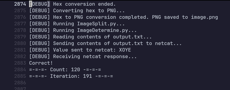
Just barely got the flag with this method. However, there is no flag… I forgot to grep for that when I hit 120 Correct Guesses. You could see from the results that this was cutting it close, considering I could not get more than 80 wrong guesses. It was only the third run where it succeeded and I’ve never felt more despair in my life.

Running the script two more times until finally 120/196:

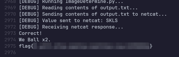
CTF solved, and somebody’s uncle got Bob’d. The final part of this CTF you ask? Well that was just to find out how to exit vim without turning off my machine and that I did. The code for this is here.

If you’re curious about “dark magic” then continue reading. After this section, was my attempt at generalising Image Classification.

Neural Networks.

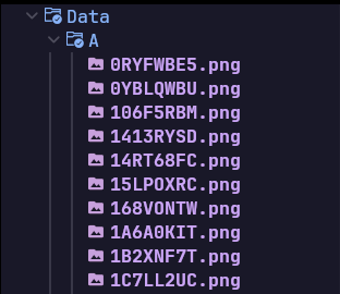
For an example let’s say we have something similar to what we have now… a folder full of images – i.e. a dataset. In this dataset we have a letter per folder – a class. In total we have 26 classes in our dataset containing one image per class, for now. Images also have pixels, which I’ll referred to as neuron. Let’s look at an image.

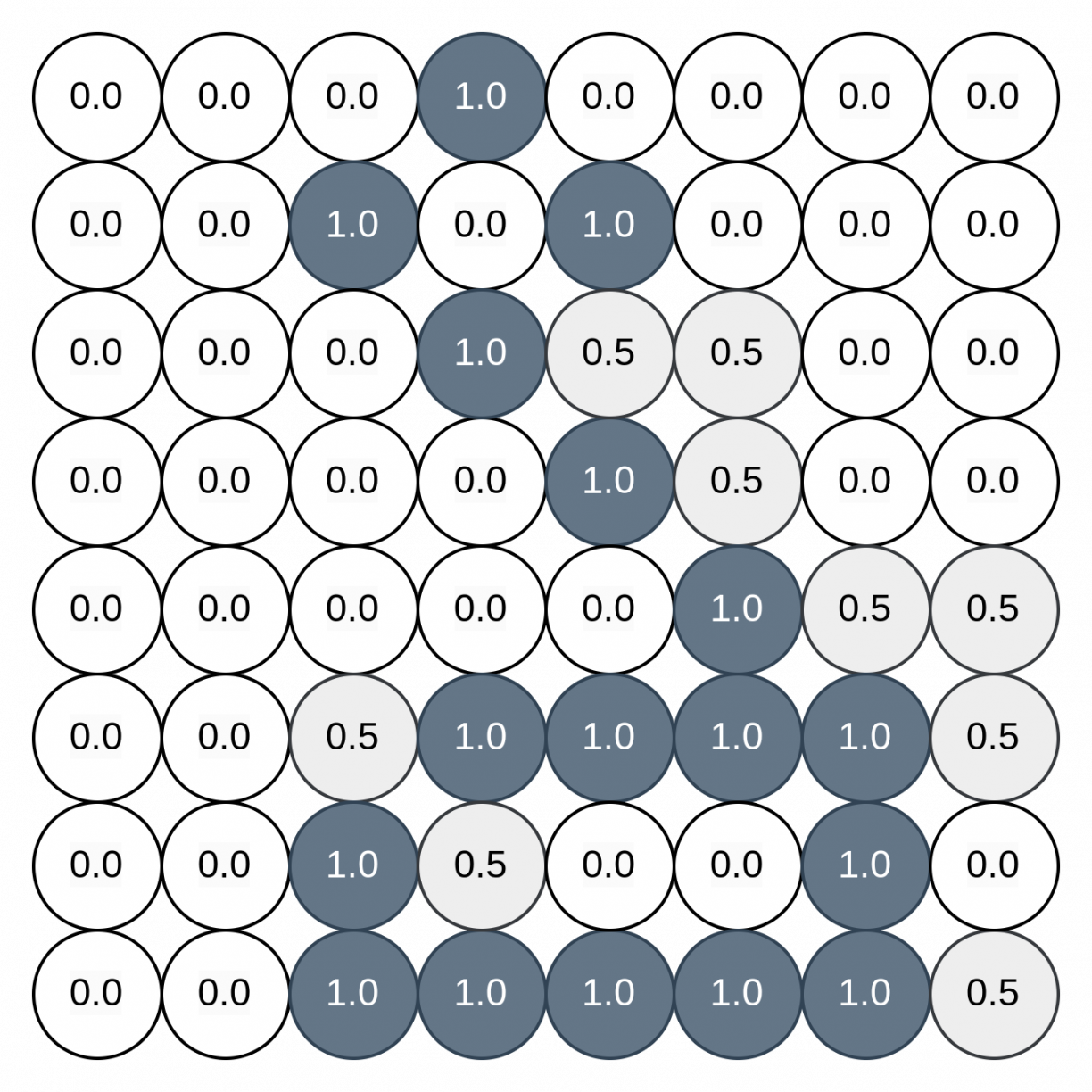
This is my example of neuron activation in an image. Each neuron has a numeric value between 1.0(ON) and 0.0(OFF). The closer to one the neuron is, the more heat or activation it has. If this image is 28×28 pixels then its has 784 neurons.

If you couldn’t tell by now this was the symbol for A in Bill Cipher. The values 0.5 are the edges of the image, think of it like the blurring effect you see in images when the definition is not as sharp. This is how images are interpreted by neural networks. So this is the “neural” part. What is the “network” part?

This is the network. The input layer is the image, which would mean that there should be 784 neurons in the input layer. Take the first screenshot of neurons and lay them out in a flat line and that would be the input layer. Layers 1, 2 and 3 we’ll come back to in a second. The output layer is the classes so there should be 26 dots to represent the results as each letter of the alphabet.

This is how the training would take place, the input layer is the image’s pixels, which goes through hidden layers 1, 2 and 3 – each determining which next point it will go to, ultimately; resulting in matching the image to the class it most likely belongs to in the output layer. 

For our example letter A would go to class 0 (First class). Layers 1, 2 and 3, point the input layer to the correct output layer. So the hidden layer would be the determining factor here. In very basic terms, the hidden layer is responsible for identifying patterns such as finding shapes.

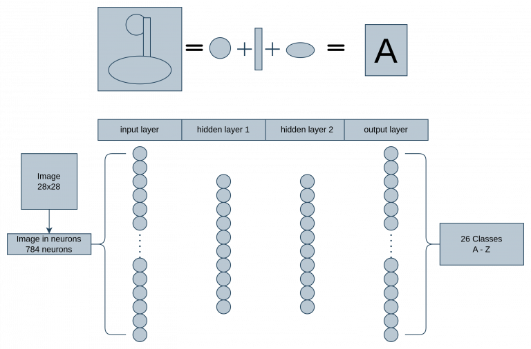
In the above you could think of it like this, the Symbol for A in Bill Cipher has certain characteristics. We would see a circle, straight line and an oval. Think of the hidden layer as identifying the shapes that make up the image. Multiple connections exist to do this, which in the end points to the most likely value in the output layer. This is of course simplified to the extreme. The “shapes” in question would look more like this, where every colour is the weight of the neuron:

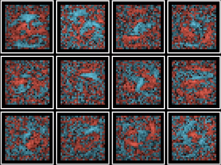
Blue neurons are positive and red would be negative values. (Note this would have 784 neurons). Think of weights as the connection to the neurons. 

An = Activation
Wn = Weights. 
(W1A1 + WnAn+ …)

The sum would be the activation range. The range of activation values is infinite negative value to an infinite positive value. But this value needs to be changed to be between or equal to 0 and 1. That’s the format of the activation range. Currently, only the weighted sum of the neuron is the activation range and to get the value between 0 and 1 we can use the sigmoid function. Sidenote: sigmoid is fairly old and has since been replaced with relu function.

s(x) = 1/(1 + e?x)
s(x)(W1A1 + WnAn+ …)

We can also add a bias from the weighted sum. i.e.: -16 is the bias. Bias is like the parameter or condition for us to define what counts as an activation, like moving something to the left or right.

s(x)(W1A1 + WnAn+ … – 16)

This now equals the pixel pattern of the hidden layer. This in turn means we now have 784 neurons, 16 weights (I just decided to make this value the same) and 16 biases. That would mean the graph would have 13 002 Weights and Biases. Sorting the weights by matrices and activation by vectors would also be:

s(x)(W1A1 + WnAn+ … + bias)

This determines the strength of the connection. This means that s(x)(W1A1 + WnAn+ … + bias) is the strength of the connection between the neurons. 

Example of a single connection.

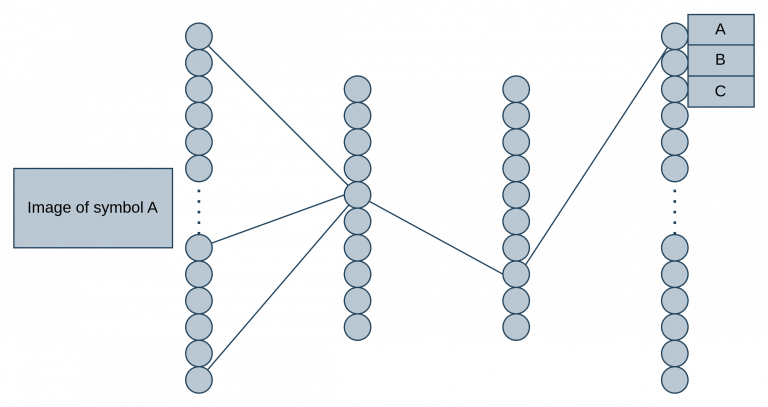
Perspective; 784 neurons, 16×2 hidden layer neurons to an output layer of 26 classes. This is also simplified to the extreme. In reality this would have multiple connections for a single image to class and the connection weights will also play a factor (The lines are the connection weights and each line will have a value).

Cool, we have all this, and what happens if we run this for the first time – disappointment. There is no correction taking place so we have to implement a cost function. That would be the output layer being told what the correct class was supposed to be. Smaller numbers are the more correct classes.

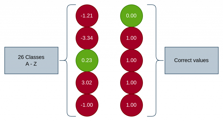
The output layer on the left is being compared to the correct values on the right for the above image. To correct the output layer we use the cost function:

(-1.21 – 0.00^2)+
(-3,34 – 1.00^2)+
( 0.23 – 0.00^2)+
(..)+
(-1.00 – 1.00) = cost

The lower the cost the more correct it is. Averages are used to measure this. 

Cost function – Weights and Biases being taken as input and class being the output. This is training data. 

C(W1, W2…W13 002) on a graph would mean the graph’s minima would be the most correct answer. In other words the lowest point in the graph. You can use slopes to determine the negative and positive shifts to find the minima. 

In this case learning means to minimise the cost function using the gradient descent. To further fine tune this, it would help to know backpropagation calculus (I don’t). Going forward and backwards in the network to improve connections. 

This is to understand the “dark magic” of what is happening behind the scenes when we use TensorFlow. I thought it was interesting how a computer “see’s” and “learns”. To make your own neural network you’ll need more than just this 101. I would recommend looking at 3blue1brown’s resources as they explain this in great detail and do a fine job at explaining it as well.

Capchan – CLI Tool to Solve CAPTCHA

Time to put it all together into a general tool – something that can be used for login brute forces on assessments. So I used my CTF script and generalised it a bit more to solve CAPTCHA’s alike.

mapping_it_out.cmapp

Before spamming “all in” pings, I like to map out what is required from my previous experiences and other issues, I noted.

Requirements:

Creating a tool in Python, based on my script I used for the CTF, that could be fed images and create a model from that. In more detail, the tool needs to be provided with folders of images where each folder represents a class. The model would be made based on what each class represents. Finally, a method of testing the model’s performance.

Pre-emptive debugging:

The issue would be model re-usability and sharing the model, similar to hashcat’s potfile. A method would be needed to generalise the data used. Another issue would be models are be specific to the properties of each image. Meaning that a model trained from smaller 28×28 RGB images would not be usable against a model that was trained with 400×500 greyscale images.

Mapping out the following for what needs to be done.

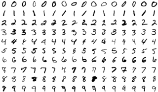
What is needed to create the model? The user would need to define a dataset by describing what classes will the images consist of. Sticking with the CAPTCHA theme, I used the MNIST database of handwritten digits to create the model. MNIST would provide images with consistent properties, which would void the possibility that one of the thousands of images could prevent my model from building as it should. The most challenging part of this is finding a method/resource to collect the images one needs, as any image too great in deference to others would break the model.

Starting: I made the model greyscale first, before implementing greater image pre-processing, which would be another challenge on its own to generalise the data given. The challenge was making all the images roughly the same, while not changing too much, which could affect the original image integrity.

Since my last venture into this topic, I’ve learned a few new things when creating a model. I’ll only mention the more important things and the unaddressed items from my CTF script. The remaining would be the collection of data and making the CLI pretty and colourful (For American English speakers, that means “colorful”).

So hyperparameters affects parameters; epochs and batches are examples, while parameters are the more internal components such as gradient descent values.

Let’s go through the parts of my final code.

As with my previous script I set a random seed to ensure that neural network (NN) does not cause issues when using the same data and model architecture. This would provide more consistent results when changing hyperparameters Think of it like making a ‘random’ script, which generates random characters. This is to void the same ‘random’ characters being generated on each run.

np.random.seed(42)
tf.random.set_seed(42)

Image generalisation, in which input_shape is set to greyscale, which will cause issues if any other image is used. i.e. a limitation FOR NOW is greyscale images, and I haven’t figured out yet how to account for this.

image_size = (224, 224)
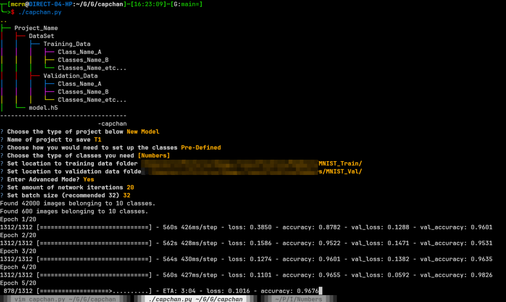
input_shape = (224, 224, 1)

Input collected, where num_classes is the amount of folders and the train_ and val_ data would be the training data and validation data. Training data is used to train the NN, while validation is used to determine the results of the current NN performance, which will affect the parameters pertaining to the gradient descents – gradient descent is used to determine minima, as minima is a “more” correct answer.

num_classes = int(custom_class_tot)
train_data_dir = custom_class_train
val_data_dir = custom_class_val

As a reminder epochs, would be a full loop of the dataset, while batch size refers to the number of images fed at a time. Meaning that 1000 images with a batch size of 10 will need 100 iterations to complete an epoch. Another example would be images equal to 3000, with batch size 32 and epoch 500 will mean 3000/32 = 94 batch loops = 1 epoch(500) = Complete model.

epochs = int(epoch_tot)
batch_size = int(batch_tot)

The tricky part of these hyperparameters is that they need to be changed based on your results, but there are restrictions. The smaller batch sizes would require more epochs and will be less accurate, while bigger batch sizes would require less, but will be prone to overfitting, where the model does great against Train/Val data and horrible against unforeseen/test data. However, batch sizes may only be in the power of two, and are required to be greater than or equal to 16.

Sidenote: I tried to find a formula that will take the amount of classes and images per class to determine the best values for hyperparameters, but most resources on NN find that there is no correlation.

The next part would be the image pre-processing. The changes to training data were kept minimal seeing as my images already vary a great deal. The validation data is not changed seeing, as it’s used to determine the cost function and will be similar to my test data when determining performance.

train_data = keras.preprocessing.image.ImageDataGenerator(
rescale=1.0 / 255,
rotation_range=1,
width_shift_range=0.1,
height_shift_range=0.1,
horizontal_flip=False
)
val_data = keras.preprocessing.image.ImageDataGenerator(
rescale=1.0 / 255
)

The following I used to generate batches of grayscale images and their corresponding labels for training the model. This will be the same for the validation data as well.

train_generator = train_data.flow_from_directory(
train_data_dir,
target_size=image_size,
color_mode="grayscale",
batch_size=batch_size,
class_mode="sparse",
shuffle=True
)

Then defining the Convolutional NN by specifying the functions to use and change other values in the array, which is mostly the same as the original CTF script

What remains is to save the model, but what I’ve change since is to create a file.cmapp (No reason for naming it .cmapp). This maps out the class number to the folder name in which it was trained in. That way, if you use other models with their generated mapping, it will allow the correct naming in the performance test, rather than it returning an integer, then having you determine what folder that integer was assigned to.

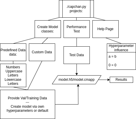
This entire process would look something like this:

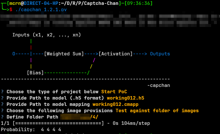
After creating the model in .h5 format and having its .cmapp be exported with it – I added a performance test, where you can use the image against other unforeseen images. This is, again, also the same as the previous CTF’s as nothing changes here. Example of what this would look like against a folder containing four number four’s:

This was the bare minimum for creating the tool, obviously there are remaining issue such as the images only being greyscale, but in terms of CAPTCHA and what this will be used for, its not that important, since the colour of the number/letter does not contribute to solving the CAPTCHA. For the future, I would still like to include other image formats to support a wider range of dataset collection. This will mean adding more to the NN to process other data differently as well as more pre-processing of images, if not already outside of this script.

I have used this on assessments in the past, where I could determine the font used for the CAPTCHA. This part is important, because knowing the font, I could create my own, similar, CAPTCHA symbols for training.

My hope for this is to keep adding on to it and by the end have a tool that could be fed images any type of image and spit out a perfect model. Remember Rice in the bowl, Windows on parole.